Assessing phylogenetic relationships of Lycium samples using RAPD and entropy theory¹

Introduction

Traditional Chinese medicine (TCM) has been used for thousands of years in China. It represents the collective wisdom of the Chinese people to utilize nature for survival^[1]. With the advantages of multi-target effects, low toxicity and the current appeal for more ‘natural’ remedies, TCM has become widely used as an alternative to treat various complex and chronic diseases. Authentication of Chinese medicinal materials is an old but important issue. With the unprece-dented development of modern biological methods, identification of species relationships using traditional anatomical and physiochemical methods is being supplemented by DNA fingerprinting techniques, such as random amplified polymorphic DNA (RAPD) analysis.

The fruit of Lycium species, especially Lycium barbarum, has been used in TCM to improve eyesight, protect liver and kidney, and to replenish vital essence. The fruit of the Lycium species are all red in color with very similar physical appearance and anatomical structure. Chemical analysis methods, such as high-performance liquid chromatography, have been used for different species of Lycium, but have failed to differentiate the Lycium species.

Recently, a Fourier-transform infrared spectroscopy method was used to identify 7 species and 3 varieties of Lycium^[2]. The method provides a novel approach for the identification and differentiation of plants used in TCM. Such a technique can serve as a rapid, simple, reliable and non-destructive analytical method for differentiating Lycium species. Alternatively, with the development of modern biotechnology, a polymerase chain reaction (PCR)-based method using random primers (10-mers), known as RAPD^[3,4], has become another method for the study of TCM^[5,6]. RAPD analysis is simple and effective. It has many advantages, such as it only requires a minute quantity of DNA; no prior sequence data are needed, many primers can be used; and the method is relatively simple. However, RAPD suffers the drawback of low reproducibility, which has severely hampered the popularity of this method. Usually, PCR products are analyzed by agarose gel electrophoresis followed by densitometric analysis of the DNA banding pattern. In the present study, the lab-on-a-chip (Agilent 2100 Bioanalyzer DNA 7500 assays, Agilent Technologies, Palo Alto, California, USA) was used to analyze the PCR products of Lycium samples, including 7 species and 3 varieties. After preprocessing using the Agilent 2100 Bioanalyzer, including baseline adjustment and alignment, data were exported as XML files, which were imported into the Matlab software. All further analyses were performed using Matlab. We will clarify these analyses in detail in the following sections.

Materials and methods

Sample preparation Twelve Lycium samples were used in this study. Dried fruits of Lycium were rinsed with 70% ethanol and distilled water for surface sterilization. They were then ground in liquid nitrogen with a mortar and pestle. Information for the samples is summarized in Table 1. Samples of Lycium barbarum, LB and LBB, were treated as positive controls in the RAPD analysis. The remaining 10 samples, which represent 7 species and 3 varieties, were used in our data analysis.

Table 1 List of Lycium species analyzed in this study.
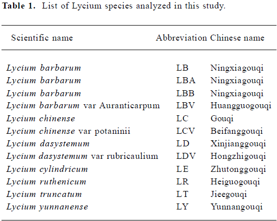
Full table

Genomic DNA extraction The cetyl triethylammonium bromide (CTAB) extraction method, a modified protocol of Draper and Scott^[7], was used for the extraction of DNA. Lycium powder was mixed with 600 µL of 1×CTAB extraction buffer [50 mmol/L Tris-HCl (pH 8.0), 0.7 mol/L NaCl, 10 mmol/L ethylenediaminetetracetic acid (EDTA), 1% CTAB], which was preheated at 60 °C. The mixture was then incubated for 30 min with occasional shaking. After cooling to room temperature, the mixture was extracted with an equal volume of chloroform/isoamyl alcohol (24:1, v/v). After centrifugation at 13 000×g for 15 min at room temperature, the supernatant was collected and a 0.1 mol/L volume of 10% CTAB solution (10% CTAB, 0.7 mol/L NaCl) and an equal volume of chloroform/isoamyl alcohol were added for another extraction. After centrifugation at 13 000×g for 15 min at room temperature, the supernatant was collected and extracted with an equal volume of CTAB precipitation buffer [50 mmol/L Tris-HCl (pH 8.0), 10 mmol/L EDTA, 1% CTAB]. It was then allowed to stand at room temperature for at least 1 h, before being centrifuged again at 13 000×g for 15 min at room temperature. The pellet was resuspended in 400 µL of 1 mol/L NaCl, which was pre-heated at 60 °C. For further purification, it was extracted again with an equal volume of chloroform/isoamyl alcohol. After centrifugation at 13 000×g for 15 min at room temperature, the supernatant was collected and 800 µL of cold absolute ethanol was added. The solution was allowed to stand at -20 °C overnight for precipitation of DNA. To recover the DNA, the suspension was centrifuged at 13 000×g for 20 min at 4 °C. The pellet was collected and washed twice with 75% ethanol. After that, the pellet was air-dried and resuspended in 30 µL distilled water.

Estimation of DNA concentration and purity The concentration and purity of DNA was checked by UV spectroscopy at wavelengths 230 nm, 260 nm, and 280 nm. The quality of DNA (5 µL) was also checked by electrophoresis on a 1% agarose gel in 1×TBE (Total Binding Energy) buffer.

RAPD and optimization of PCR conditions The RAPD reactions were carried out as described by Nadeau et al^[8] in a 25 µL reaction mixture containing DNA (10 ng–100 ng), 0.1 mmol/L dNTP, 25 pmol primer, 1×Taq buffer [20 mmol/L (NH₄)₂SO₄, 75 mmol/L Tris-HCl (pH 8.8), 0.01% Tween-20, 2.5 mmol/L MgCl₂, 0.001% gelatin (w/v)] and 0.5 U Taq DNA polymerase. The tubes were placed in the thermocycler (PTC-100^TM, MJ Research Inc Waltham, Massachusetts, USA) and subjected to the following profiles: denaturation for 5 min at 94 °C, then 45 cycles at 94 °C for 1 min, 35 °C for 1 min, 72 °C for 2 min, final extension at 72 °C for 5 min. In order to optimize the RAPD conditions, the PCR conditions were varied using 100-fold, 500-fold, 1000-fold and 5000-fold dilutions of genomic DNA, 2 mmol/L or 2.5 mmol/L MgCl₂, 1 U or 1.25 U Taq polymerase in the presence or absence of the final extension step. The PCR products were monitored by 1.5% agarose gel electrophoresis and the DNA fragments were visualized by staining with ethidium bromide. The amplification products (1 µL) were also analyzed with the lab-on-a-chip system, the Agilent 2100 Bioanalyzer, using the DNA 7500 assays kit according to the manufacturer’s instructions.

Results

Preprocessing of raw data Raw lab-on-a-chip DNA fingerprints can be treated as multi-dimensional vectors or functional curves. Because they are usually observed and stored discretely, in the present study, the vector form was adopted to represent the DNA fingerprint. We let (t_i, x_i), i=1, ..., T denote the discrete observations for a DNA fingerprint, where x_i is the fluorescence intensity measured at migration time t_i and T is the number of migration time points. Customarily, fluorescence intensity is referred while ommitting migration time in representing DNA fingerprint, namely, (x₁, ..., x_T) represents a fingerprint, where a is the transpose of a vector for a.

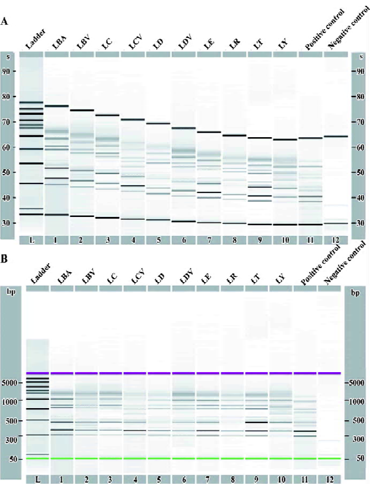
A complete preprocessing for raw fingerprint data includes baseline adjustment, alignment, linear interpolation match and normalization issues. In order to eliminate the background and peak drift effect for DNA fingerprints, we used the up-to-date Agilent 2100 Bioanalyzer^[9] software to adjust baseline and handle alignment based on the ladder, lower marker and upper marker. Figure 1 shows the alignment process.

Figure 1 RAPD fingerprints of 10 Lycium samples (1–10), two control samples (11, 12) and ladder sample (L) obtained from primer opam2 performed by Agilent 2001 Expert software. (A) Fingerprints without alignment; (B) aligned fingerprints.

After baseline adjustment and alignment, we exported the data into an XML format, which could be opened by Microsoft Excel. The XML files were then imported by the software Matlab, which was our main tool for further analysis. It was easy to detect the lower marker and upper marker that define the informative region for each fingerprint. Therefore, we could concentrate on the observations between the lower and upper markers. However, fingerprint data after baseline adjustment and alignment was shown with relative migration time, which was different from the unaligned data, that is, fingerprint data with the same length of interval between the lower marker and upper marker but with different number of migration time points. Here linear interpolation was used to match all of the fingerprints such that they had the same number of migration time points between the lower marker and upper marker. This method is called linear interpolation match (LIM). Our main purpose for using LIM was to render the fingerprints directly comparable. Another reason was to make the data format suitable for our statistical analysis. Details about the LIM method are described using Lycium samples as follows.

After exporting Lycium sample data from Agilent 2100 Expert software, the total 110 fingerprints produced by 11 primers and the corresponding number of migration time points were denoted by x_i(k) and n_k,j,k=1, ..., 11; i=1, ..., 10. Because these fingerprints shared the common interval between the lower marker and the upper marker, we first chose the minimum number {n_k,j}, denoted as m, and then made the migration time points the same for all of the other fingerprints in the following way. We uniformly partitioned m–1 cells on interval [0,1]. Similarly, for any fingerprint that had s migration time points, we uniformly partitioned s–1 cells on interval [0,1]. The total migration time points corresponded to 0, 1/(s-1), 2/(s-1), ..., 1. For any i/(s-1), 0<i<s-1, we found j such that i/(s-1) located on an exclusive interval [j/(m-1), (j+1)/(m-1)]. Liner interpolation of the fluorescence intensity value at corresponding retention time j/(m-1) and (j+1)/(m-1) was changed to the i-th fluorescence intensity value for the newly matched fingerprint. Following the above rule, all of the fingerprints were matched with the same number of migration time points. After performing LIM, the common peaks of both ends, which were parts of the lower and upper markers, were removed as these peaks were of no concern. For simplicity, the number of migration time points of these fingerprints was still noted as T.

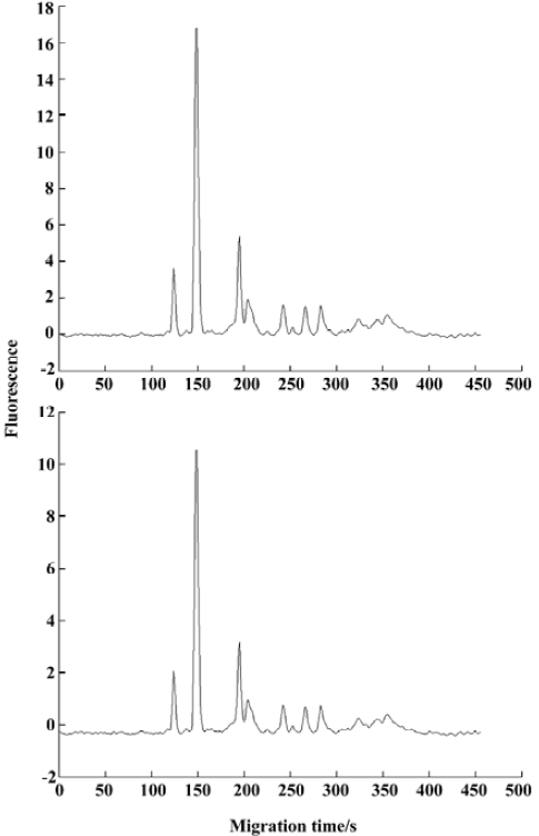
Because the outcomes of most statistical methods are strongly influenced by the scale and range of the fingerprint data, it was necessary to normalize all of the fingerprint data before analysis. To accomplish this goal, the sample mean and variance of the fingerprint x=(x₁, ..., x_T)' were calculated as follows:

All of the fingerprints were normalized by subtracting the sample mean and then dividing by the standard deviation, namely the following form:

The effect of this normalization is shown in Figure 2. From then on, fingerprint i referred to the registered fingerprint after normalization.

Figure 2 Normalization effect on fingerprints. (A) Fingerprint before normalization; (B) fingerprint after normalization.

Primer sorting by the revealed fingerprint diversity DNA fingerprinting performed by RAPD using different primers may have had different detected diversities. The diversity of fingerprints obtained from a primer, what we call dispersivity, can be regarded as an index to indicate whether this primer is effective or not. As an example, for our tested DNA fingerprints of Lycium samples representing 7 species and 3 varieties, all DNA fingerprint data were denoted by:

X=(X⁽¹⁾, ..., X⁽¹¹⁾),

where X^(k)=(X₁^(k), ..., X₁₀^(k)), k=1, ..., 11, k denotes k-th primer, and the total primer number 11, 10 denotes the total number of Lycium samples, namely, 7 species and 3 varieties. X_i^(k) is a T-dimensional column vector that denotes the fingerprint of Lycium sample from species i obtained from primer k. T is the number of migration time points. Initially, the information about dispersivity revealed by primer k was contained in the data set X^(k). Usually the more peaks in the data set X^(k) obtained form primer k, the higher the dispersivity. However, that is not always true because the difference in peak location and the variation in peak height and peak shape among fingerprints obtained from primer k can also affect the corresponding dispersivity. It is necessary and important to integrate all of the factors in the evaluation of the dispersivity for each fingerprint set X^(k).

In the present study, we used the concept of entropy, introduced by Shannon and Weaver^[10], to quantify the dispersivity revealed by primer k. For a discrete probability distribution p, the motivated definition of entropy by statistical mechanics is:

were . In the context of probability, h(p) is regarded as a measure of the information carried by p, with high entropy corresponding to much uncertainty. This uncertainty score reflects the property of dispersiity. Intuitively, it manifests itself as the way we describe dispersivity.

The dispersivity revealed by primer k is defined as the following way:

Step 1. Compute the sample covariance matrix

where

Step 2. Calculate the eigenvalues of S^(k) and note them as λ^(k)=(λ₁^(k), ..., λ₁₀^(k))'

Step 3. Make the sum of eigenvalues equal to 1, namely,

Setp 4. Compute entropy of λ^(k), namely,

h(λ^(k)) is defined as the dispersivity revealed by the primer k. The definition of dispersivity is very intuitive. In the first step, we used the covariance matrix S^(k) to describe all of the variant information for the fingerprints obtained from primer k. The variant information was then extracted by computing the eigenvalues of S^(k). These eigenvalues, λ^(k), can be regarded as the information reconstructed from X^(k) and can be interpreted by the principal component analysis (PCA). Sort λ₁^k, ..., λ₁₀^k as λ₍₁₎^(k) ≥ .. ≥ λ₍₁₀₎^(k), for the fixed primer k, the closer to 1 for

which can be considered as the contribution rate for the first principal component, the stronger for the first principal component to synthesize the information of X^(k). For example, if fingerprints l₁^(k), ..., l₁₀^(k) are very similar, it will result in the contribution rate for the first component being close to 1 and the sum of the remaining 9 being near to 0, which means that the first component can synthesize almost all of the information. This case is not expected, because it reflects little diversity for X^(k). We desired that the contribution rates for all of the components were scattered, not concentrated, and allowed for the entropy, which has the property that the more dispersive it is for the probability distribution, the larger the corresponding entropy value. Finally, we defined the dispersivity revealed by primer k as

Here all the λ_j^(k) denote the contribution rates subject to the sum being equal to 1. From the definition of dispersivity, some eigenvalues may be equal to 0, which will result in no meaning due to the function. In such cases, we defined 0×ln(0)=0, which is reasonable because λ×ln(λ) will approach 0 if λ approaches 0 from the positive direction.

For our Lycium data, 11 primers were used to perform the analysis. A direct question is which primer is the best one as far as dispersivity is concerned? To some extent, the best primer would be able to differentiate the Lycium samples to the maximum degree. The dispersivity revealed by primer k was given by h(λ^(k)), simply noted as D(X^(k))=h(λ^(k)), where λ^(k) is dependent on X^(k). The best primer was chosen as the one that maximized the value of D(X^(k)). Memory the best primer and the corresponding dispersivity value as S1 and D_S1, respectively.

After choosing the primer S1, we then wanted to choose a second primer from the remaining 10, such that the fingerprints obtained from these 2 primers had the maximum diversity. In order to do this, we had to define the dispersivity of the 2 primers. For a striking example, if fingerprints X⁽ⁱ⁾ and X^(j) obtained from primers i and j, respectively, were very similar, that would mean that primers i and j almost revealed the same dispersivity. Furthermore, if primer i revealed the maximum dispersivity and primer j revealed the second maximum dispersivity, then primer i would be picked as the best primer, while in most cases, primer j would not be selected as the primer that reveals the maximum diversity combined with primer i, because X⁽ⁱ⁾ and X^(j) have much mutual information. This indicated to us that we should remove overlapping information before choosing primers from the remaining 10. The method of space projection was utilized to solve the information overlap.

The dispersivity revealted by primers i and j, on condition that primer i was chosen, was defined as D(X⁽ⁱ⁾,(1-X⁽ⁱ⁾(X⁽ⁱ⁾)⁺)X^(j)), where A⁺ denotes the pseudoinverse of matrix A^[11] and can be numerically calculated by Matlab. The computation of D(A,B) was similar to D(A) except for substituting A union B for A. For simplicity, we define CP(X⁽ⁱ⁾|X^j)=(1-X⁽ⁱ⁾(X⁽ⁱ⁾⁺)X^j. Matrix CP(X⁽ⁱ⁾|X^j) was corthogonal to the space expanded by X⁽ⁱ⁾. That means that it contained extra information relative to X⁽ⁱ⁾. The eigenvalues of covariance matrix for X⁽ⁱ⁾ union CP(X⁽ⁱ⁾|X^j) were the union of eigenvalues of covariance matrix for X⁽ⁱ⁾ and CP(X⁽ⁱ⁾|X^j). For our Lycium data, on the condition that primer S1 was chosen, the second primer cosen was he one that corresponded to the maximum value of D(X^(S1),CP(X^(S1)|X^(k)), k∈{1,2, ..., 11}/{S1}, were A/B denotes the set that includes the elements belonging to A but not to B. Without loss of generality, the second primer chlosen is recorded as S2, the corresponding dispersivity value is denoted by D_S1,S2.

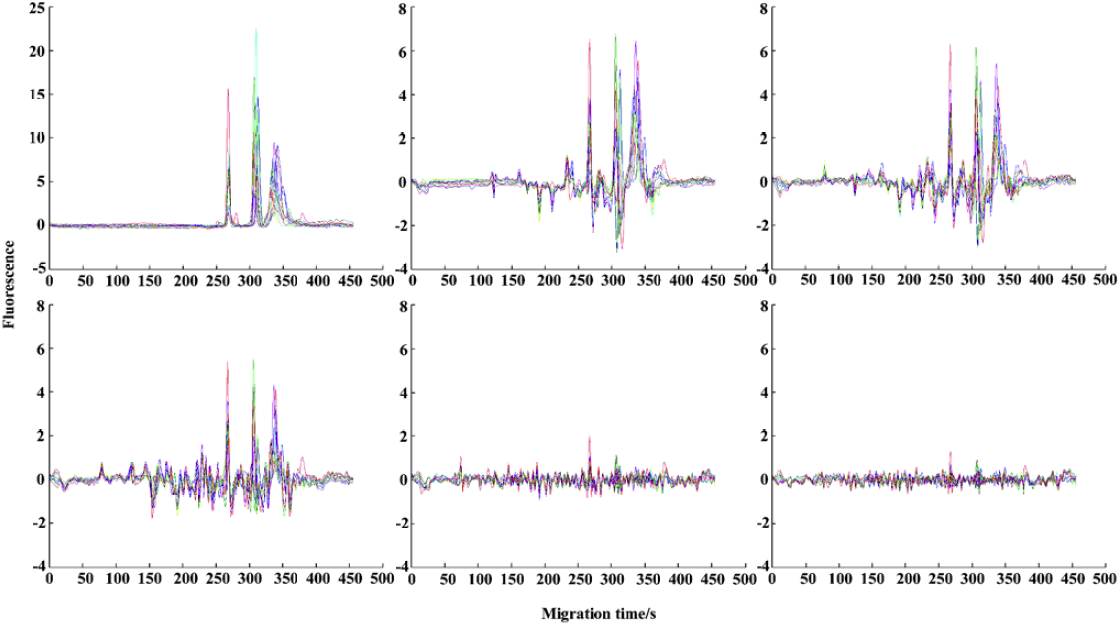
We could then obtain the order of primers, denoted S1, ..., S11. The corresponding dispersivities for the primers were denoted D_S1, ..., D_{S1, ..., S11}. For illustrating our space projection method, in Figure 3, we plot the original fingerprint for primer S9, namely, X(S9), extra information relative to primer S1, namely, CP(X^(S1)|X^S9), and extra information relative to primers S1, ..., S8, namely, CP{X^(S1), CP(X^(S1)|X^(S2)), ..., CP[X^(S1), CP(X^(S1)|X^(S2), ..., CP(X^(S1)|X^(S8))]}|X^(S9). Comparing the plots in Figure 3, the information provided by primer S9 gradually decreased as the mutual parts relative to primers chosen earlier S1, ..., S8 were removed one by one. This property can be interpreted by the projection theory and Figure 3 is an intuitive manifestation.

Figure 3 Fingerprints obtained from primer S9 and extra information relative to the earlier-picked primers. (A) Original fingerprints for primer S9; (B) extra information relative to primer S1; (C) extra information relative to primers S1,S2; (D) extra information relative to primers S1,S2,S3; (E) extra information relative to primers S1, …, S7; (F) extra information relative to primers S1, …, S8.

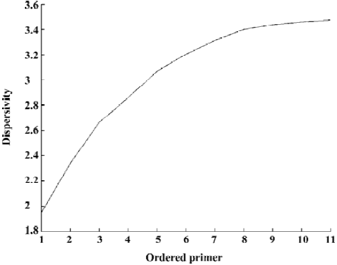
Construction of the dendrogram for Lycium samples From Figure 4, the x coordinate denotes the primers according to the order in which they were chosen and the y coordinate denotes the corresponding dispersivity. For example, 2 denotes primers S1 and S2, and the corresponding y-value is D_S1,S2, which shows that the dispersivity increases as the newly chosen primer is added. Furthermore, the extent of the increase becomes smaller and smaller. That means that adding a primer can increase the amount of information available while the last primer chosen provides less information than the previous primer. Generally, the more primers chosen, the better the conclusion drawn, such as in distinguishing and constructing the dendrogram for our Lycium samples of 7 species and 3 varieties. However, because the last primers chosen provided relatively little information, it was not necessary to pick all 11 of the primers to construct the dendrogram. In the present study, we decided on the primer number that contained almost all of the information to distinguish and construct the dendrogram for Lycium samples using argmin(D_{S1, ..., Si})/(D_{S1, ..., S11})>95%. For our Lycium samples, (D_{S1, ..., S11})'=(1.9476, 2.3398, 2.6624, 2.8600, 3.0690, 3.2071, 3.3133, 3.3998, 3.4380, 3.4611, 3.4772)'. The number of primers to use can be obtained by simple computation according our proposed rule. Because, (3.2072/7.3772)=0.9223<0.95, (3.3133/3.4772)=0.9529>0.95, 7 primers, S1, ..., S7, were chosen for final analysis. We used the 95% rule to decide the number of primers. Generally, in most data analyses (such as PCA) it is possible to use other rules, for example, the 80% rule, to decide the number of principal components. However, we used the larger number 95% because our proposed dispersi-vity is a sensitive index. This means that the dispersivity changes only a small amount, while the fingerprint changes much. It is therefore better to widen the boundaries for choosing in case some important primers are lost.

Figure 4 Plot of {(i, D_{S1, ..., Si})} for Lycium samples.

In the present study, we used the hierarchical cluster method to construct a dendrogram of Lycium species. Because each Lycium sample was analyzed using 7 primers, the primer information was merged by weighting. The weights were assigned by ω₁=D_S1/D_{S1, ..., S7}, ω_k=(D_{S1,..., Sk}-D_{S1, ..., S(k-1)})/D_{S1, ..., S7}, k=2, ..., 7. Using the obtained weights of primers, the distance of each Lycium sample from species i and j was defined by:

were

d(x_i^(k), x_j^(k))=1-ρ²(x_i^(k), x_j^(k)),

s(x_i^(k), x_j^(k)) and s(x_i^(k)) are defined by (5) and (2). ρ(x_i^(k), x_j^(k)) is the correlation coefficient between x_i^(k) and x_j^(k), which is often used to measure the similarity of fingerprint. In order to use distance matrices to onstruct the dendrogram, we transformed the data by 1-ρ(x_i^(k), x_j^(k))².

Unweighted pair-group method using arithmetic average (UPGMA) linkage, which defines the cluster distance, is advocated for constructing a dendrogram. Details about the UPGMA clustering method can be found in Sokal and Michener^[12]. Using the above distance measure between fingerprints and the UPGMA cluster method, we visualized the cluster results using the dendrogram shown in Figure 5.

Figure 5 Dendrogram of 10 Lycium samples using the first 7 primers ordered.

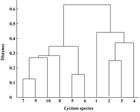
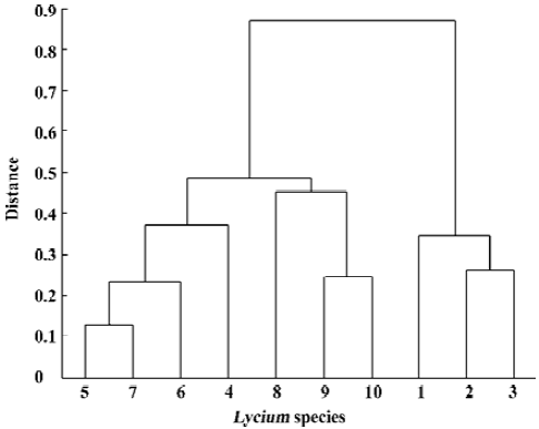
For evaluating our procedure to decide the number of primers, we used primers S1, ..., S8 to construct the dendrogram as above, further more, we use the first ordered 9, 10, and 11 primers to construct dendrogram, respectively. All of these were similar to Figure 5. This indicated that the first 7 primers contained almost all of the information provided by the total 11 primers. Furthermore, when using primers S1, ..., S6, the outcome shows little difference relative to Figure 5 (Figure 6). It manifests our picking procedure for primer number is so delicate.

Figure 6 Dendrogram of 10 Lycium samples using the first 6 primers ordered.

Discussion

Phylogenetic relationship construction based on RAPD fingerprint data generated from a number of primers was investigated in this study. We proposed an index called dispersivity using entropy theory to describe the diversity of RAPD fingerprints obtained by several primers. Generally, this index can be applied to other DNA fingerprint data, such as arbitrarily primered PCR and DNA amplification finger-printing, and to chromatographic fingerprints, such as chromatogram, spectrum and mass spectrum. Based on this index, the order for choosing primers is obtained using the orthogonal projection method and entropy theory. Our proposed method provides the guidelines for primer picking in the consequent experiments. An on-line analysis program on RAPD primer selection is provided on the web site: http://math.nenu.edu.cn/shiz/yinxiaolin.files/program.htm, which can be downloaded easily if required.

Acknowledgements

We are grateful to Dr Daniel KWONG (the Chemistry Department of Hong Kong Baptist University) for his valuable comments on the manuscript.

References

1. Chan K, Lee H. The way forward for Chinese medicine. London: Taylor and Francis; 2002.
2. Peng Y, Sun SQ, Zhao ZZ, Leung HW. A rapid method for identification of genus Lycium by FTIR spectroscopy. Spectrosc Spect Anal 2004;24:679-81.
3. Welsh J, McCelland M. Fingerprinting genomes using PCR with arbitrary primers. Nucleic Acids Res 1990;18:7213-8.
4. Williams CE, Ronald PC. PCR template-DNA isolated quickly from monocot and dicot leaves without tissue homogenisation. Nucleic Acids Res 1994;22:1917-8.
5. Shaw PC, Wang J, But PPH. Authentication of Chinese medicinal materials by DNA technology. London: Word Scientific Publishing; 2002.
6. Zhang AJ, Wong NS, Ha WY, Hu YH, Fang KT. Authentication of traditional Chinese medicines using RAPD and functional polymorphism analysis. In: Fang KT, Liang YZ, Yu RQ, editors. Proceedings of the 1st Conference on Data Mining and Bioinfor-matics in Chemistry and Chinese Medicines; 2003 Apr 6–16; Shenzhen, China; 2003. p 81–98.
7. Draper J, Scott R. Plant genetic transformation and gene expres-sion. London: Blackwell Scientific Publishing; 1988.
8. Nadeau JH, Bedigian HG, Bouchard G, Denial T, Kosowsky M, Norberg R, et al. Multilocus markers for mouse genome analysis: PCR amplification based on single primers of arbitrary nucleotide sequence. Mamm Genome 1992;3:55-64.
9. Agilent []: Agilent Technologies. 2100 Bioanalyzer Expert User’s Guide; c2000-2005 [updated 2004 Mar 1; cited 2005 May 10]. Available from: http://www.home.agilent.com
10. Shannon CE, Weaver W. The mathematical theory of com-munication. Urbana, IL: University of Illinois Press; 1949.
11. Rao CR, Mitra SK. Generalized inverse of matrices and its applications. New York: Wiley; 1971.
12. Sokal RR, Michener CD. A statistical method for evaluating systematic relationship. Univ Kans Sci Bull 1958;28:1409-38.