Support vector machine for SAR/QSAR of phenethyl-amines¹

Introduction

The structure-activity relationship (SAR) and the quantitative structure-activity relationship (QSAR) studies are basically concerned with the correlation of structure with activity. Many different statistical methods, such as the multiple linear regression (MLR)^[1] and partial least squares (PLS) analysis^[2] have been employed to SAR/QSAR analyses. Several physicochemical descriptors, such as hydrophobicity, topology, electronic parameters, and steric effects, are usually used in QSAR studies. Recently, many researches have been concerned with applying the support vector machine (SVM) to investigate SAR/QSAR^[3–7]. The SVM, a statistical approach mentioned by Vapnik^[8] and developed in the last decade, has lately started to be applied in this field. The potential of SVM for use in SAR/QSAR has been discussed^[9–15]. In this work, beta-adrenergic agonists and antagonists (phenethyl-amines) are studied with the application of SVM in the field of SAR and QSAR. Beta-adrenergic agonists and antagonists are well known for their enhanced effect on the growth hormone-releasing hormone (GHRH)-induced growth hormone (GH) secretion in human bodies. They are significant mediators on the GH response to GHRH in anorexia nervosa^[16–19]. As SVM is a robust tool in the SAR/QSAR field, our objective is to study the modeling of phenethyl-amines by SVM to classify antagonists/agonists and predict the activity. To demonstrate the power of SVM, computations were performed by the cross-validation^[20] and independent test, which are deemed the most rigorous and objective test procedures in statistical prediction. As the number of samples in this work is very small, the independent test and a special cross-validation, leave-one-out cross validation (LOOCV), were used to test the models’ generalization and reliability^[21].

Materials and methods

Support vector classification Support vector classification (SVC) has been recently proposed as a very effective method for solving pattern recognition problems. SVC is a learning machine based on statistical learning theory. The basic idea of applying SVM to pattern classification can be stated briefly as follows^[3,22]: suppose we are given a set of samples, that is, a series of input vectors x_i∈R^d (i=1, ..., N) with corresponding labels (x₁, y₁), ..., (x_m, y_m), ..., y∈{-1, +1}; where -1 and +1 are used to stand, respectively, for the 2 classes. The goal here is to construct 1 binary classifier or derive 1 decision function from the available samples, which has a small probability of misclassifying a future sample. In other words, the goal is to seek an optimized linear division, that is, construct a hyperplane, w^Tx+b=0 that separates the 2 classes (this can be extended to multi-classes). Different mappings construct different SVM. The mapping x_i∈R^d (i=1, ..., N) is performed by a kernel function:

K(x_i, x_j)=Φ(x_i)Φ(x_j) (1)

which defines an inner product in the space H.

The decision function implemented by SVM can be written as:

where the coefficients α_i are obtained by solving the following convex quadratic programming problem:

In Equation 4, C is a regularization parameter which controls the trade-off between the margin and misclassification error.

These x_j are called support vectors only if the corresponding α_i>0. Several typical kernel functions are:

K(x_i, x_j)=(x_i·x_j+1)^d (5)

K(x_i, x_j)=exp(-γ || x_i –x_j ||²) (6)

Equation 5 is the polynomial kernel function of degree d which will revert to the linear function when d=1. Equation 6 is the radial basic function (RBF) kernel with 1 parameter γ.

The SVM training process always seeks a global optimized solution and avoids over-fitting, so it has the ability to deal with a large number of features. A complete description to the theory of SVM for pattern recognition is given by Vapnik^[22].

Support vector regression (SVR)^[3,22] Support vector regression (VM) can be applied to regression by the introduction of an alternative loss function and the results appear to be very encouraging. For the case of regression approxima-tion, suppose there is a given set of data points

(x_i is input vector and is the desired value). SVR is based on the structural risk minimization principle from the statistical learning theory. Each instance is represented by a vector x with molecular descriptors as its components. A kernel function, K(x_i, x_j), is used to map the vectors into a higher dimensional feature space, and linear regression is then conducted in this space. The optimal regression function can be represented by:

where l is the number of support vectors and the coefficients α_i, α_i* and bias b are determined by maximizing the following Lagrangian expression:

with the following constrains:

0≤ α_i ≤C i=1, ..., l

0≤ α_i* ≤C i=1, ..., l

where l is the training set size and C is a penalty for training errors.

Leave one out cross-validation (LOOCV) During the process of LOOCV, both the training dataset and testing dataset are actually open and a sample will in turn move from one to the other. Each sample in the dataset is in turn singled out as a tested sample and all the rule-parameters are calculated based on the remaining samples. In other words, each sample is predicted by the rule parameters derived using all the other samples except the one which is being predicted^[20–21].

Sensitivity analysis Sensitivity analysis (SA) is the study of how the variation in the attributes of a model can be apportioned, qualitatively or quantitatively, to different targets of variation. A mathematical model is defined by a series of equations, input factors, attributes, and variables aimed to characterize the process being investigated. Good modeling requires an evaluation of the confidence in the model, possibly assessing the uncertainties related to the modeling process and with the outcome of the model itself. SA offers a valid method for characterizing the uncertainty associated with a model. The model is run for a set of sample points for the attributes of concern or with straightforward changes in the model structure. This approach is often used to investigate how the target changes significantly in relation to the changes of attributes. The application of this approach is straightforward, and it has been widely employed in nonlinear modeling^[23,24]

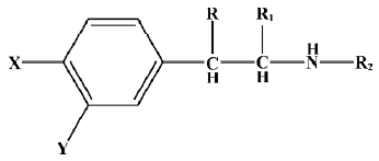
Data sets and descriptors The compounds with various substituents (X, Y, R, R₁, and R₂)^[25] are shown in Figure 1. The structural details and the activity class of 32 chosen phenethyl-amine compounds are given in Table 1. Seventeen of these are antagonists (class 1) and fifteen are agonists (class 2). The data set is divided into the training set and the testing set.

Figure 1 Structure of the phenethyl-amines.

Table 1 Substituents X, Y, R, R₁, and R₂.
Full table

The substituents in the phenyl group were described by the fragment constant value of Tekker (f)^[26], electronic parameters of Taft (σ)^[27], STERIMOL parameters (L and B) and the electronic parameters of Hammett (E_S)^[28], plus the calculated pKa of the amino group.

Owing to the redundancy of some parameters, the selection of descriptors for a SAR/QSAR study is necessary, but not straightforward^[29]. However, the selection of descriptors will contribute a lot to construct the actual model. Recently, promising results have been reported on the problem of feature selection^[29–31]. Generally, the presence of irrelevant or redundant features can cause the model to lose sight of the broad picture that is essential for generalization beyond the training set. In particular, this problem is compounded when the number of observations is also relatively small. The main goal of feature selection is to select a subset of d features from the given set of D measurements (d<D) without significantly degrading the performance of the mathematical model. In this work, the global searching method was applied to the selection based on descriptors which were used in Wold’s study^[25]. Prediction accuracy was calculated with different combinations of the descriptors. Based on the calculation results, we will choose the descriptors with the best prediction accuracy. Therefore, 4 selected descriptors (pKa, fR2, σR2, and Σ-p) were found suitable to construct the SVC model; 3 selected descriptors (pKa, fR2, and E_sR2) were found suitable to construct the SVR model for the activities of agonists, and 4 selected descriptors (fPh, fR2, fR1, and B4) were found suitable to construct the SVR model for the activities of antagonists. Further combinations of descriptors may exist which may be useful for the SAR/QSAR study of the data set used here, but the selected subset proved to be appropriate for a successful prediction of activities, therefore we did not look for further sets.

Results

Classification model-based SVC of the antagonist and agonist

Selection of kernel function and the capacity parameter C It is well known that similar to other multivariate statistical models, the performance of SVC is related to dependent and independent variables, as well as the combination of parameters used in a model. In the computation of SVC, the capacity parameter C (or regularization parameter) and the kernel type used in modeling must be selected.

In this study, the suitable capacity parameter C and the kernel function type in building the model were selected based on the LOOCV method. The accuracy of prediction (P_A) in LOOCV was employed as a criterion in selection. P_A can be computed as follows:

where N_T is the number of samples in the whole data set and N_C is the number of samples whose classes are correctly predicted in LOOCV.

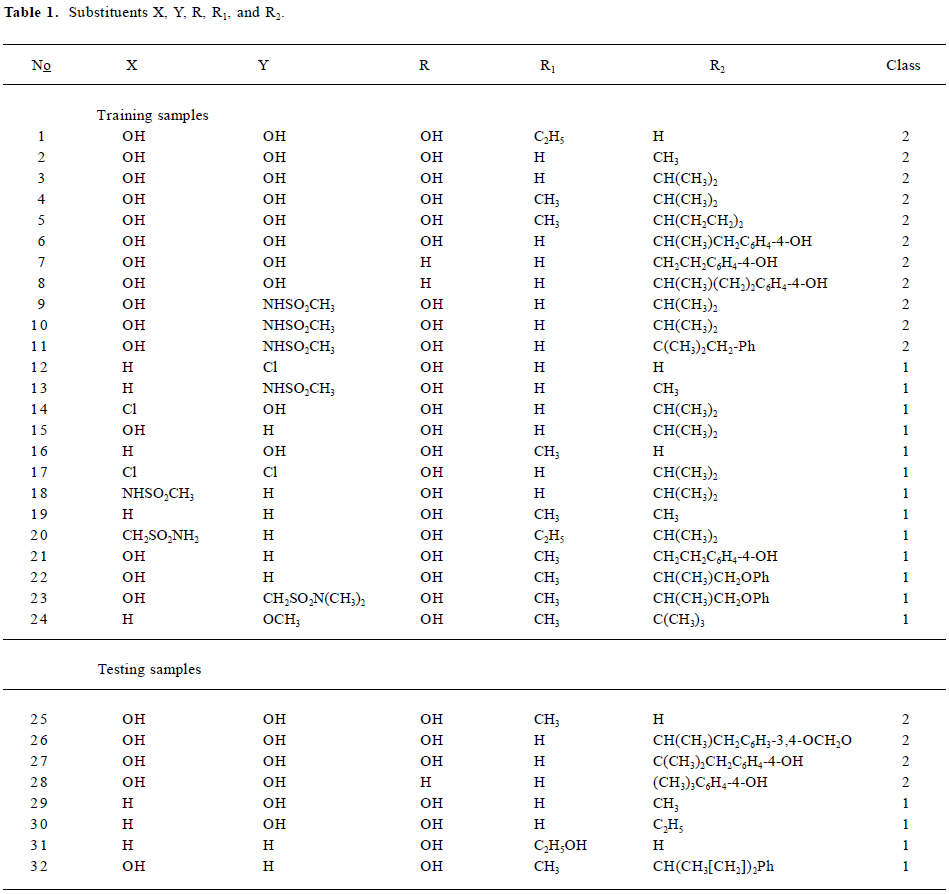
Figure 2 shows the curve of P_A versus the capacity para-meter C (its value from 1 to 200) with different kernel functions (linear and polynomial radial basis functions) by using SVC LOOCV. It can be seen in Figure 2 that P_A gets maximal value employing the RBF kernel function with the capacity parameter C≥146. Gamma (g) is another parameter of SVC which will affect the prediction capacity when using the RBF kernel function. Hence, we calculated the prediction accuracy under different C and g (for RBF). Figure 3 shows the P_A versus C (C=1–200, step=1) and g (g=0.1–3, step=0.1) with the RBF kernel function. From Figure 3 we can see that although g affected the prediction accuracy, the maximal value of P_A is 91.67%. In this case, g was set as default value 1. So the SVC model with best performance could be expected by using the RBF kernel function with the capacity parameter C=146, g=1.

Figure 2 P_A vs C by using SVC LOOCV.

Figure 3 P_A vs C and g by using SVC-RBF LOOCV.

Modeling of SVC According to the results obtained from above section, the optimal model of SVC for discriminating antagonists from agonists is as follows, using RBF kernel function with the capacity parameter C=146, g=1:

where x is a vector (pattern of sample) with unknown activity to be discriminated and x_i is one of the support vectors.

According to Equation 11, the compounds could be discriminated as antagonists if g(x)≥0 and the accuracy of classification (C_A) is 95.83%.

C_A can be defined as follows:

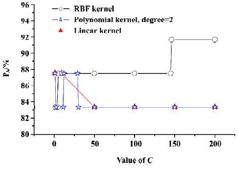
where N_T is the number of samples in the whole data set and N_C is the number of samples which are discriminated correctly. Figure 4 shows the effect of classification with the trained SVC model. It demonstrates that only 1 sample is classified incorrectly.

Figure 4 Trained effect of classification with SVC.

Results of LOOCV for classification The predictive ability was evaluated by the accuracy of prediction (P_A) in LOOCV.

Figure 5 shows the effect of prediction validated by the LOOCV method. In Figure 5, there are also only 2 samples predicted incorrectly, and the accuracy of prediction (P_A) is 91.67%. Additionally, to compare with the prediction generalization ability of SVC method, the Fisher method, the K-nearest neighbor (KNN, K=5), and the artificial neural network (ANN), with 3 hidden nodes and Sigmoid transformation function were also applied in this work, with the prediction accuracies were 75%, 83.33%, and 79.17% in the LOOCV test, respectively.

Figure 5 Effect of prediction with LOOCV test of SVC.

Results of independent test for classification To validate the generalization and reliability of the classification model (Equation 11), the independent test set was employed in this study. The accuracy of prediction is 100%. The Fisher method, the KNN, K=5, and the ANN were also applied in this work, and the prediction accuracies were 87.5%, 75%, and 75% in the independent test, respectively.

Predicting the activity of phenethyl-amines SVM models relate not only to the task of distinguishing between pairs of molecules based on SVC, but the task of predicting actual biological activity based on SVR. Just like the SVC method, the performance of SVR in predicting the activity is also related to dependent and independent variables, as well as the combination of parameters used in a model. In the computation of SVR, the capacity parameter C, the epsilon insensitive loss function (ε), the gamma (g), and the kernel type used in modeling must all be selected. In this computa-tion, the least root mean square error (RMSE) in LOOCV was employed as the criterion to obtain the appropriate kernel function and the optimal capacity parameter C, ε, and g. RMSE is defined as follows:

where e_i is the experimental value of sample i, p_i is the predicted value of sample i in the LOOCV of SVR, and n is the number of the total samples. In general, the smaller the value of RMSE obtained, the better predictive ability expected.

As the mechanisms of antagonists’ and agonists’ activity are different, their QSAR models would be built respec-tively.

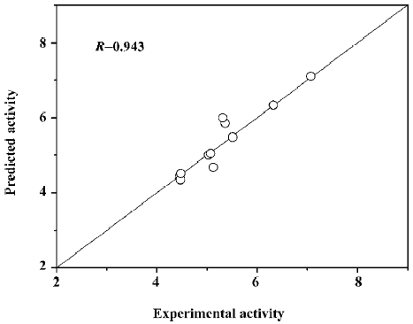
Optimal SVR model for antagonists To obtain the suitable modeling parameters, the RMSE was calculated under different parameters (ε, C, and g) and different kernel functions (including the linear kernel function, the polynomial kernel function, and the RBF kernel function) by using the LOOCV of SVR. Figure 6A–6E shows the effects of RMSE with different kernel functions and different parameters. Figure 6A illustrates RMSE versus C (C=0.1–200, step=0.1) and ε (ε=0.01–0.3, step=0.01) with the linear kernel function. Figure 6B illustrates RMSE versus C (C=0.1–200, step=0.1) and ε (ε=0.01–0.3, step=0.01) with the polynomial kernel function. Figure 6C illustrates RMSE versus C (C=0.1–200, step=0.1) and ε (ε=0.01–0.3, step=0.01) with the RBF kernel function. Figure 6D illustrates RMSE versus g (g=0.1–3, step=0.1) and ε (ε=0.01–0.3, step=0.01) with the RBF kernel function. Figure 6E illustrates RMSE versus C (C=0.1–200, step=0.1) and g (g=0.1–3.0, step=0.1) with the RBF kernel function. After comparing the above plots, the author found that the RBF kernel function is better than both the linear function and poly function in the building model. Hence, according to Figure 6, the optimal SVR model for antagonists can be presented as follows, with the RBF kernel function (C=0.5, ε=0.1, and g=1.4):

Figure 6 RMSE in LOOCV vs C and Epsilon with linear kernel function (A), polynomial kernel function (B), and RBF kernel function (C). RMSE in LOOCV vs g and Epsilon with RBF kernel function (D) and Epsilon with RBF kernel function (E).

ACT=Σ(α_i − α_i*)×exp[-1.400×|| x − x_i^* ||²]+0.471 (13)

where (α_i − α_i*) is the Lagrange coefficient corresponding to the support vector. Figure 7 illustrates the relationship of predicted activities and the experimental activities of agonists, with R=0.943.

Figure 7 Correlation of experimental and predicted activity of agonists using Equation 13.

Optimal SVR model for agonists In this section, the data set of agonists was investigated by the same method used for antagonists. Figure 8A–8E shows the effects of RMSE with different kernel functions and different para-meters.

Figure 8 RMSE in LOOCV vs C and Epsilon with liner kernel function (A), poly kernel function (B), and RBF kernel function (C). RMSE in LOOCV vs C and g with RBF kernel function (D) and RBF kernel function (E).

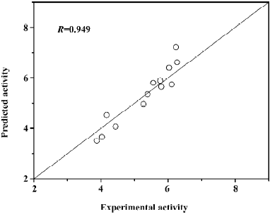
According to Figure 8, the optimal SVR model for agonists can be presented as follows, with the RBF kernel function (C=1.9, ε=0.01, and g=1.4):

ACT=Σ(α_i − α_i*)×exp[-1.400×|| x − x_i^* ||²]+0.223 (14)

where (α_i − α_i*) is the Lagrange coefficient corresponding to the support vector. Figure 9 illustrates the relationship of predicted activities and the experimental activities of antagonists, with R=0.949.

Figure 9 Correlation of experimental and predicted activity of antagonists using Equation 14.

Results of LOOCV of SVR In order to further confirm our findings, we investigated the relationships between experimental and predicted activity values. The detailed experimental values and calculated values are given in Table 2. These relationships are shown in Figure 10A,10B, which illustrates the effect of prediction with the aforementioned model (Equations 13 and 14) validated by the LOOCV method. Figure 10 suggests that the predicted activities are in agreement with experimental activities for agonists and antagonists, with correlation (R) 0.831 and 0.865, respectively.

Table 2 Predicted activities with different method using LOOCV.
Full table

Figure 10 Correlation of experimental and predicted activities of agonists (A) and antagonists (B) in LOOCV test of SVR (using RBF kernel).

MLR, PLS regression (PLSR), and ANN were also utilized to predict the activities of phenethyl-amine compounds with special consideration of their generalization abilities in the LOOCV test compared to SVR. The calculated results are given in Table 2. The RMSE in the LOOCV test using SVR, MLR, PLS, and ANN, respectively, are listed in Table 3. It can be found that the generalization ability of SVR is superior to the other methods which are often used in QSAR studies in the LOOCV test.

Table 3 RMSE of agonist/antagonist activity in LOOCV test of SVR, MLR, PLS, and ANN.
Full table

Results of independent SVR test As a demonstration of practical application, predictions were also conducted for the independent data set based on the models derived from the training data set. MLR, PLSR, and ANN were also utilized to predict the activities of phenethyl-amine compounds with special consideration of their generalization abilities in the independent test compared to SVR. The calculated results are given in Table 4. Table 5 lists the RMSE in the independent test using SVR, MLR, PLS, and ANN, respec-tively. It can be found that the generalization ability of SVR is superior to the other methods which are often used in QSAR studies.

Table 4 Predicted activities with different method using independent test.
Full table

Table 5 RMSE of agonist/antagonist activity in independent test of SVR, MLR, PLS, and ANN.
Full table

Discussion

Parameters It is important to set the adjustable parameters of SVR to obtain the model with the better, or at least sufficient, predictive capability. Parameter C is an important parameter because of its possible effects on the trade-off between maximizing the margin and minimizing the training error. If the value of C is too small, then insufficient stress may be placed on fitting the training data. If the value of C is too large, then the algorithm may over-fit the training data. From Figures 6 and 8, we can see that if C >100 or C<0.01, the value of RMSE will be very large, which means that the prediction accuracy of activity will be very poor. The optimal value of ε is another important parameter. ε prevents the entire training set meeting boundary conditions, and so allows for the possibility of sparsity in the dual formulation’s solution. Hence, choosing the appropriate value of ε is critical from theory, but it is hard to find an appropriate value of ε as there is no rule as to how to optimize it. In this study, we predict the value of RMSE while the range of ε is 0.001–0.31, and we found that if the value is smaller, the result will be better. However, it will take more time when the value of ε is very small. The optimal value of g also plays a significant role in this study. g controls the amplitude of the Gaussian function, therefore controls the generalization ability of SVM. In this study, the prediction accuracy of activity changed greatly when g ranged from 0.1 to 3; when the value of g was out of this range, the result was poor. The parameters should be optimized together with the kernel functions type adopted in SVR modeling.

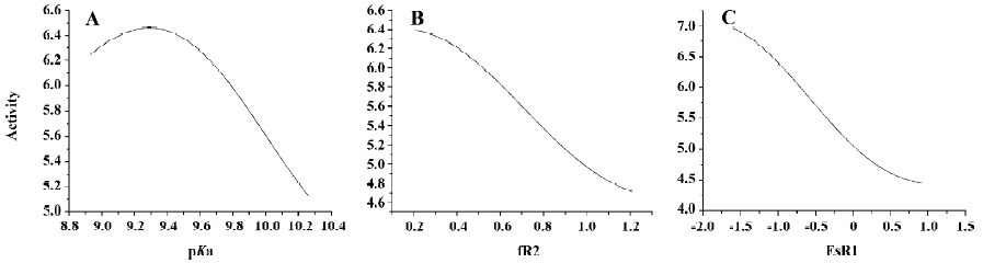
Sensitivity analysis (SA) In this paper, 2 QSAR models of phenethyl-amines are attained with highly accurate predictions. However, the aforementioned models are nonlinear, and it is hard to analyze the relationship between attributes and activity. Hence, we used the sensitivity analysis to study how the attributes affect the target.

SA of QSAR model of agonists From Figure 11A, we can see that when the values of fR2 and ESR1 are fixed, the value of activity varies with the increase of pKa, and a maximum value of activity exists when the value of pKa is around 9.4. From Figure 11B, we can see that when the values of pKa and ESR1 are fixed, the value of activity will decrease with the increase of fR2. From Figure 11C, we can see that when the values of pKa and fR2 are fixed, the value of activity will decrease with the increase of ESR1. According to these findings, we can conclude that decreasing the value of ESR1 and fR2 and choosing the value of pKa around 9.4 will result in higher activity of agonists.

Figure 11 (A) activity vs pKa by SA; (B) activity vs fR2 by SA; (C) activity vs EsR1 by SA.

SA of QSAR model of antagonists From Figure 12A, we can see that when the values of fR2, fR1, and fPh are fixed, the value of activity will increase with the increase of B4. From Figure 12B, we can see that when the values of B4, fR1, and fPh are fixed, the activity varies with the increase of fR2, and a maximum value of activity exists when the value of fR2 is around 0.95. From Figure 12C, we can see that when the values of B4, fR2, and fPh are fixed, the value of activity will increase with the increase of fR1. From Figure 12D, we can see that when the values of B4, fR1, and fR2 are fixed, the value of activity will decrease with the increase of fPh. According to these findings, we can conclude that there if we want to get higher activity of antagonists, maybe we can increase the value of B4 and fR1, decrease the value of fPh, and choose a proper value of pKa around 0.95.

Figure 12 (A) activity vs B4 by SA; (B) activity vs fR2 by SA; (C) activity vs fR1 by SA; (D) activity vs fPh by SA.

Advantages and disadvantages of SVM Compared with other algorithms used in chemometrics, SVM has outstanding advantages: it can be used for both classification (SVC) and regression (SVR); it is suitable for both linear and nonlinear problems; it has special generalization ability, especially for problems of small sample size; and it has no local minimum problem. As a newly-proposed algorithm, SVM has a bright future as a powerful tool for chemistry and related fields owing to these advantages. The investigations presented here show that the SVM technology is a robust and highly accurate, intelligent classification and regression technique which can be successfully applied to deriving statistical models with good statistical qualities and good predictive capabilities within areas, well suited to SAR/QSAR analyses of drug research.

Although SVM outperforms PLS, MLR, and ANN techniques in this study, different machine-learning algorithms would have their own advantages and disadvantages in different data sets. In fact, the different approaches may provide complementary information from different point of views, and sometimes the combination of different methods may result in better results than the single one for special data sets. Despite the advantage of SVM, adjusting the parameters is hard work and affects the application of SVM. However, no general guidelines are available to select these parameters. The approach we used in this study is time-consuming and there are possibly still better parameters than the ones we employed. Hence, developing an efficiency method to adjust the parameters is important in future work.

In this work, the SAR and QSAR analyses based on the SVM method for 32 phenethyl-amines was studied, and 1 SAR and 2 QSAR models were developed. The predictive powers of these models were verified with the LOOCV test and independent test methods. For the LOOCV test, the accuracy of the classification using Equation 11 with LOOCV was 91.67%. The RMSE for antagonists using Equation 13 was 0.5881, and the RMSE for agonists using Equation 14 was 0.4779. For the independent test, the accuracy of the classification using Equation 11 with LOOCV was 100%. The RMSE for antagonists using Equation 13 was 0.3727, and the RMSE for agonists using Equation 14 was 0.1435. Taking the promising results made above into account, it could be concluded that the SVM method could be employed to SAR/QSAR modeling with much improved quality and predictability.

Appendix

The calculations were implemented on a 1830 MHz Centrino Duo computer (Dell, Xiamen, China), running the Windows XP operating system (Microsoft, Redmond, USA). All the learning input data were range-scaled to (0, 1) in this work. The SVM software package named ChemSVM including SVC/SVR, was programmed in our lab^[32–34].The validation of the software has been tested in some applications in chemistry and chemical technology^[33,34].

Acknowledgement

The authors wish to thank Dr Beke TAMÁS for reading this manuscript and improving its presentation.

References

1. Draper NR, Smith H. Applied regression analysis. New York: Wiley; 1998.
2. Wold S, Johansson E, Cocchi M. PLS-partial least-squares projections to latent structures, 3D QSAR in Drug Design. Leiden,ESCOM, 1993.
3. Zhao H, Lu WC. Support vector machine applied to the pattern recognition of guanidines as Na/H exchange inhibitors. Comput Appl Chem 2002;19:691. Chinese..
4. Chen NY, Lu WC, Liu X. On the relationships between geometrical parameters of polycyclic aromatic hydrocarbons and their environmental properties. Comput Appl Chem 2002;19:749. Chinese..
5. Lu WC, Wang K, Chen NY. Support vector machine. The pattern recognition of activity of antagonists. Comput Appl Chem 2002;19:741. Chinese..
6. Dong N, Lu WC, Chen NY, Zhu YC, Chen KX. Using support vector classification for SAR of fentanyl derivatives. Acta Pharmacol Sin 2005;26:107-12.
7. Lu WC, Dong N, Naray-Szabo G. Predicting anti-HIV-1 activities of HEPT-analog compounds by using support vector classification. QSAR Comb Sci 2005;24:1021-5.
8. Vapnik VN. Statistical learning theory. New York: John Wiley and Sons; 1998.
9. Burbidge R, Trotter M, Buxton B, Holden S. Drug design by machine learning: support vector machines for pharmaceutical data analysis. J Comput Chem 2001;26:5-14.
10. Czerminski R, Yasri A, Hartsough D. Use of support vector machine in pattern classification: application to QSAR studies. Quant Struct Act Relat 2001;20:227-40.
11. Demiriz A, Bennett KP, Breneman CM, Embrechts MJ. Support vector machine regression in chemometrics. 33 rd Symposium on Computing Science and Statistics: Proceedings of Interface. E-Business Department, Verizon Inc. 2001, June.
12. Zernov VV, Balakin KV. Drug discovery using support vector machines. The case studies of drug-likeness, agrochemical-likeness, and enzyme inhibition predictions. J Chem Inf Comput Sci 2003;43:2048-56.
13. Xue CX, Zhang RS, Liu HX, Yao XJ. An accurate QSPR study of O-H bond dissociation energy in substituted phenols. J Chem Inf Comput Sci 2004;44:669-77.
14. Luan F, Zhang RS, Zhao CY. Classification of the carcinogenicity of N-Nitroso compounds based on support vector machines and linear discriminant analysis. Chem Res Toxicol 2005;18:198-203.
15. Luan F, Ma WP, Zhang XY, Zhang HX, Liu MC, Hu ZD, et al. Quantitative structure-activity relationship models for prediction of sensory irritants (logRD₅₀) of volatile organic chemicals. Chemosphere 2006;63:1142-53.
16. Gianotti L, Arvat E, Valetto MR. Effects of beta-adrenergic agonists and antagonists on the growth hormone response to growth hormone-releasing hormone in anorexia nervosa. Biol Psychiatry 1998;43:181-7.
17. King JF, Grant A, Keirse MJNC, Chalmers I. Beta-mimetics in preterm labour: an overview of the randomized controlled trials. Br J Obstet Gynaecol 1988;95:211-22.
18. Canadian preterm labor investigators group. Treatment of preterm labor with the beta-adrenergic agonist ritodrine. N Engl J Med 1992;327:308-12.
19. Mukherjee C, Caron MG, Mullikin D, Lefkowitz RJ. Structure-activity-relationships of adenylate cyclase-coupled beta-adrenergic receptors: determination by direct binding studies. Mol Pharmacol 1976;12:16-31.
20. Chou KC, Zhang CT. Prediction of protein structural classes Crit Rev Biochem Mol Biol 1995;30:275-349.
21. Schulerud H, Albregtsen F. Many are called, but few are chosen. Feature selection and error estimation in high dimensional spaces. Comput Methods Programs Biomed 2004;73:91-9.
22. Gunn SR. Report No ISIS 1998.1-98.
23. Errico RM, Vukicevic T. Sensitivity analysis using an adjoint of the PSU-NCAR mesoscale model. Mon Weather Rev 1992;120:1644-60.
24. Cacuci DG. Sensitivity theory for nonlinear systems. I. Nonlinear functional analysis approach. J Math Phys 1981;22:2794-802.
25. Wold S, Dunn III WJ, Hettbeg S. In Drug Design: Fact or fantasy. London: American Press; 1984; 94–117.
26. Rekker RF. The hydrophobic fragment constant. Amsterdam: Elsevier; 1977.
27. Taft RW. In steric effects in organic chemistry. New York: Wiley; 1956.
28. Verloop A, Hoogenstraaten W, Tipker J. In: Ariens EJ, editor. Drug design; vol VII. New York: Academic Press; 1976. 165–7.
29. Li GZ, Wang ZX, Yang J, Yao LX, Chen NY. A SVM-based feature selection method and its applications. Comput Appl Chem 2002;19:703-5. Chinese..
30. Dash M, Liu H. Feature selection for classification. Intell Data Anal 1997;1:131-56.
31. Chen NY, Qin P, Chen RL, Lu WC. Pattern recognition applied to chemistry and chemistral industry. Beijing: Science Press; 2000. Chinese.
32. Smola AJ, Schölkopf B. A tutorial on support vector regression. Stat Comput 2004;14:199-222.
33. Chen NY, Lu WC, Yang J, Li GZ. Support vector machine in chemistry. Singapore: World Scientific Publishing Company; 2004.
34. Lu WC, Chen NY, Ye CZ, Li GZ. Introduction to the algorithm of support vector machines and software. Comput Appl Chem 2002;19:697-702. Chinese..